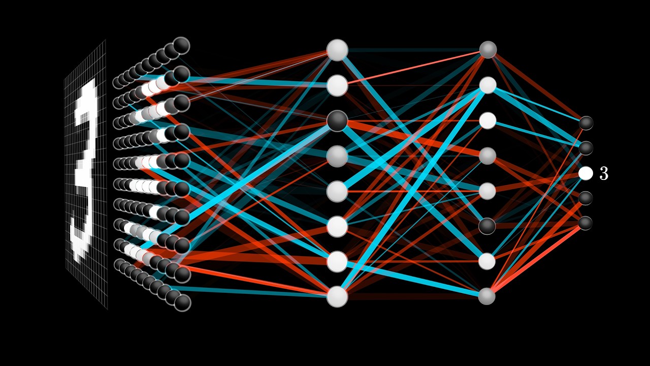
The handwriting recognizer of the app
is the main focus of this blog.
The model is a Residual Convolutional Neural Network.
Deep learning framework used: JAX
        ┏ input image
        ┃  64 × 64 × 1
        ┃       ↓
        ┃  3×3 convolution
        ┃  1 → 8 channels
        ┃       ↓
        ┃  64 × 64 × 8
        ┃       ↓
        ┃ ┌──────────────────────────────┐
        ┃ │ Residual Block × 2           │
        ┃ │                              │
        ┃ │  3×3 convolution             │
        ┃ │       ↓                      │
        ┃ │  Group Normalization         │
        ┃ │       ↓                      │
        ┃ │  ReLU                        │
        ┃ │       ↓                      │
        ┃ │  3×3 convolution             │
        ┃ │       ↓                      │
        ┃ │  Group Normalization         │
        ┃ │       ↓                      │
        ┃ │  + skip connection           │
        ┃ │       ↓                      │
        ┃ │  ReLU                        │
        ┃ └──────────────────────────────┘
        ┃       ↓
        ┃  64 × 64 × 8
        ┃       ↓
        ┃ 2×2 Max Pool
        ┃ stride = 2
        ┃       ↓
        ┃  32 × 32 × 8
        ┃       ↓
        ┃ channel change
        ┃  3×3 convolution
        ┃  8 → 16 channels
        ┃       ↓
        ┃  32 × 32 × 16
        ┃       ↓
        ┃ ┌──────────────────────────────┐
        ┃ │ Residual Block × 2           │
        ┃ │                              │
        ┃ │  3×3 convolution             │
        ┃ │       ↓                      │
        ┃ │  Group Normalization         │
        ┃ │       ↓                      │
        ┃ │  ReLU                        │
        ┃ │       ↓                      │
        ┃ │  3×3 convolution             │
        ┃ │       ↓                      │
        ┃ │  Group Normalization         │
        ┃ │       ↓                      │
        ┃ │  + skip connection           │
        ┃ │       ↓                      │
        ┃ │  ReLU                        │
        ┃ └──────────────────────────────┘
        ┃       ↓
        ┃  32 × 32 × 16
        ┃       ↓
        ┃ 2×2 Max Pool
        ┃ stride = 2
        ┃       ↓
        ┃  16 × 16 × 16
        ┃       ↓
        ┃ channel change
        ┃  3×3 convolution
        ┃  16 → 32 channels
        ┃       ↓
        ┃  16 × 16 × 32
        ┃       ↓
        ┃ ┌──────────────────────────────┐
        ┃ │ Residual Block × 2           │
        ┃ │                              │
        ┃ │  3×3 convolution             │
        ┃ │       ↓                      │
        ┃ │  Group Normalization         │
        ┃ │       ↓                      │
        ┃ │  ReLU                        │
        ┃ │       ↓                      │
        ┃ │  3×3 convolution             │
        ┃ │       ↓                      │
        ┃ │  Group Normalization         │
        ┃ │       ↓                      │
        ┃ │  + skip connection           │
        ┃ │       ↓                      │
        ┃ │  ReLU                        │
        ┃ └──────────────────────────────┘
        ┃       ↓
        ┃  16 × 16 × 32
        ┃       ↓
        ┃ Flatten
        ┃       ↓
        ┃  8192 features
        ┃       ↓
        ┃ Fully Connected
        ┃       ↓
        ┃  48 outputs
        ┃       ↓
        ┃ Log Softmax
        ┃       ↓
        ┗  48-class prediction
Since I was going to spend time making it, I wanted it to be something useful. But my main goal was educational rather than maximizing performance. I think the best way to understand something deeply is to make it from scratch and that was exactly what I set out to do.
This is the probably the most important but most tedious part of a CNN.
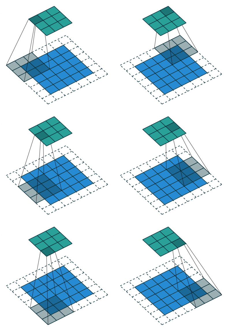
Coding the convolution (right image), however, can be somewhat tedious. The bottom square is a 7x7 square. This can be thought of a 6x6 input image with 1 pad on all sides. Here it will be defined as \(X\) The square can be though of as the output feature map \(F\). The GIF above (right image) shows the application of a 3x3 kernel \(K\) on the input image \(X\).
Directly translating the equation into code using for loop for each row, column per kernel can however be extremely slow to run. Not only is the for loop slow, your are only doing dot products of 3x3 matrices and calling the GPU each time.
I overcame this issue by isolating the patch extraction and the calculation. In the illustration above for instance, I would initially extract the patches \(P\). Here I relied on a function in jax called jax.lax.conv_general_dilated_patches to extract all the patches in advance.
Then I did the calculations at once using einsum.
\(P \in \mathbb{R}^{3\times3\times9} \) (the gif shows 9 patches) \( \quad K \in \mathbb{R}^{3\times3\times n} \) (if I used n kernels)9 (m) is \(3^2\) so I have a 3x3 feature map for each kernel. Exactly the same result as the first equation! Except this time, all the for loop are handled by a patch extraction function that is written by pros. The calculations are done at once with only one GPU call making it more parallelizable.